

The productivity quotient
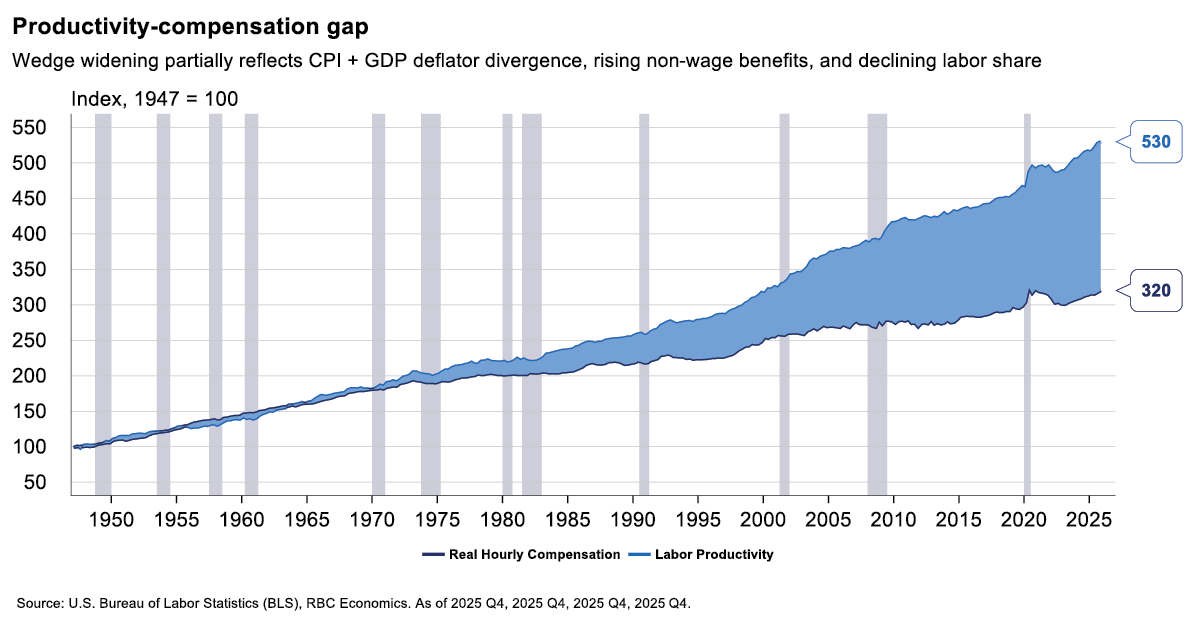
Productivity measures how efficiently the US converts capital and labor inputs into the economy’s output of goods and services.
Understanding the exact construction of US productivity metrics is essential in an environment characterized by persistent labor market tightness along with the accelerating integration of artificial intelligence and broader capex spending.
Productivity is a foundational measure that establishes the sustainability of corporate profit margins, anchors the long-term trajectory of interest rates, and benchmarks the maximum sustainable growth rate of an economy without triggering inflation.
While conceptually simple (output divided by hours worked), the official Bureau of Labor Statistics (BLS) metric requires navigating a complex, inter-agency data pipeline including inputs from the Bureau of Economic Analysis (BEA), US Census Bureau, and multiple BLS divisions. The BEA constructs real gross domestic product and sectoral value-added numbers (numerator), and the BLS performs the final index aggregation. The Current Employment Statistics (CES) establishment survey, National Compensation Survey (NCS), and Current Population Survey (CPS) are used to construct the hours worked denominator.
This guide deconstructs the architecture, clarifies common misconceptions, and helps to explain ambiguities in the measurement.
Looking ahead: The AI paradigm shift
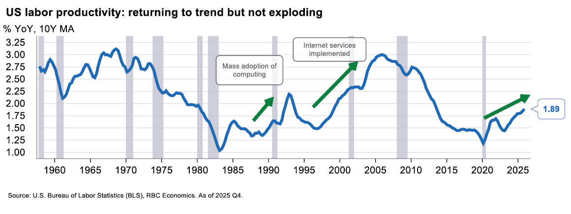
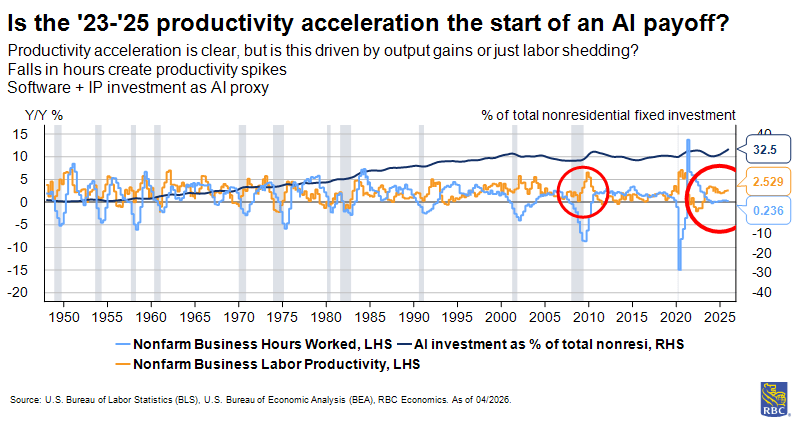
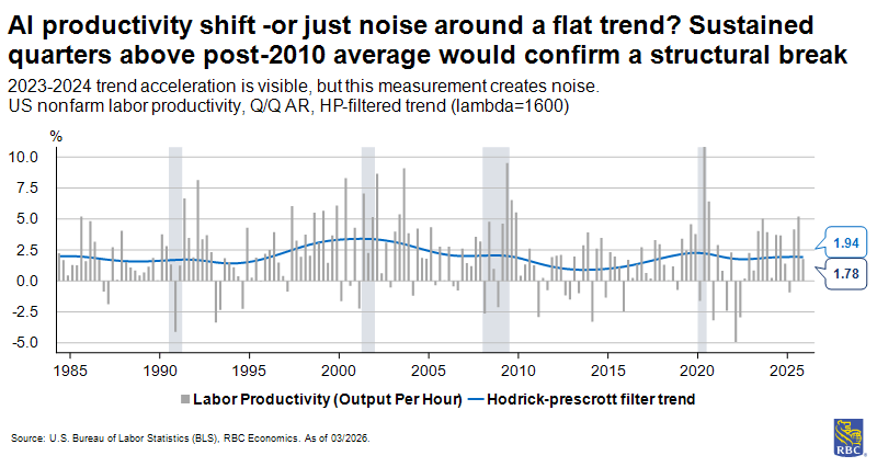
The central question for productivity analysts in 2026 is whether the measured acceleration in nonfarm business output per hour — which reached 1.9% y/y at the end of 2025, still below the roughly 2.1% average from 1950 through 2019 — represents an AI-driven structural inflection or another episode of cyclical mechanisms producing a temporary signal. One explanation for the current situation—new technologies widely recognized as impactful yet absent from aggregate macro data—claims that general purpose technologies such as electricity, the internal combustion engine, computing, and now AI, share a common adoption pattern. They all require large complementary investments in intangible capital, including retraining, workflow redesign, organizational restructuring, and new business processes, before their productivity gains materialize. These intangible investments are front-loaded and are not fully captured in the output numerator during the build phase, because the output gains accrue only after the reorganization is complete. The result is a measured productivity slowdown during the investment phase, followed by acceleration once the complementary capital is in place, hence, the J-curve shape.
The historical parallel is electrification. The adoption of electric motors in US manufacturing began in the 1890s, but the productivity gains did not appear in economic measurements until the 1920s, after factory layouts had been reorganized around distributed electric power rather than the hydraulic and steam-based machinery. The 30-year lag between technology introduction and productivity gains is not the expected J-curve timeline for AI, as our technology diffuses faster, and the complementary organizational changes are less capital-intensive. Nonetheless the basic dynamic applies.
The current data is encouraging but interpretively difficult. BLS nonfarm business labor productivity growth appears to have accelerated since 2023 and would be consistent with the early phase of the J-curve. Unfortunately, downward revisions to Q4 GDP growth undermine earlier analyses that had been cited as evidence of productivity acceleration, a reminder that measurement nuances are currently operating in ways that could inflate or deflate the measurement. It is still premature to conclude that a structural shift is happening. The post-2022 tech sector layoff cycle has improved composition effects in the information sector. The post-pandemic services recovery has been uneven, creating composition noise in aggregate figures. Also, AI deployment is concentrated in a small number of frontier firms and sectors, meaning the aggregate BLS series may understate the potential inflection by averaging AI-adopter gains with the much larger non-adopter base.
The sector-by-sector implications of the J-curve framework vary substantially. Information has the shortest expected J-curve horizon: a primary labor input (software development) is directly automatable, the measurement process (quality adjustments) is the most detailed, and the sector’s own firms are building the AI infrastructure they simultaneously deploy (shortened J-curve). Finance and Insurance has a medium-term horizon: back-office assistive technologies in surveillance, fraud detection, and report generation are already utilized. Retail Trade is also a likely early mover as demand forecasting, inventory optimization, and fulfillment automation could directly reduce input requirements per unit of output in ways would appear relatively quickly in productivity statistics. Manufacturing, healthcare, and construction represent progressively longer horizons, not because AI has less potential, but because the measurement of each sector is less capable of detecting the gains. The organizational restructuring required before gains materialize is more complex, physical, and capital-intensive. The J-curve for AI in healthcare may be the longest of any sector in the economy: even if AI diagnostics and workflow automation genuinely reduce input per patient outcome, the visit-and-procedure- count output measure will not record the gain in improved outcomes. Importantly, as healthcare continues to grow as a share of the overall economy, this means that the overall impact to productivity could be more muted than appreciated due to the changing industry mix.
The BLS produces two primary types of productivity statistics
-
Single-factor productivity (labor productivity)—the ratio of output to labor input alone.
-
Total factor productivity (TFP) —accounts for capital, energy, materials, and purchased services.
Labor productivity is defined as the ratio of real output to labor hours for the nonfarm business sector to track how productivity changes over time.
The BLS uses a growth method that treats increases and decreases symmetrically, meaning a 10% rise followed by a 10% decline returns you to the starting point. This approach, while unintuitive, makes it easier to compare productivity changes across different time periods.
Labor productivity is a single-factor approach, attributing all output growth to labor input alone, which is straightforward and enables quick assessments. But it conflates efficiency improvements with increased investments in machinery that make workers more productive. In these situations, labor productivity rises even without technological innovation, they simply have more tools.
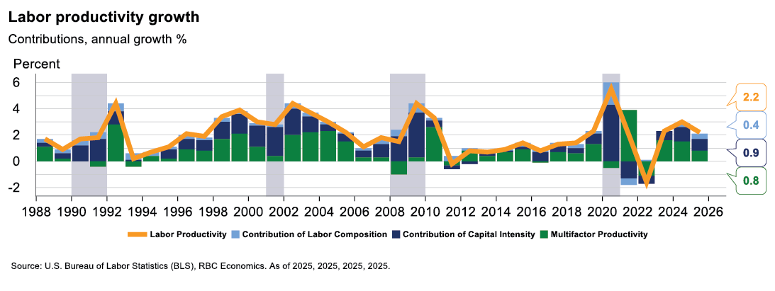
TFP is used to explain labor productivity growth in greater detail by isolating input growth from efficiency and technological gains.
It allocates output across an index of various observable inputs, adding capital and intermediate inputs to labor as production factors. Once TFP is broken out, labor productivity growth is explained by three factors: TFP growth (e.g., technological and organizational improvements, synergies, better management, and other unmeasured factors), capital intensity (e.g., greater quantity of capital, more equipment per worker), and labor composition (e.g., more human capital in the workforce, more experience, sectoral composition).
The numerator: Aggregating output
The BLS measures output using real output minus intermediate inputs—a concept known as real value-added output sourced from the BEA.
BLS uses this to create an index of output that is similar, but distinct from topline GDP. This prevents double-counting of resource inputs throughout the supply chain. As an example, when an auto manufacturer purchases steel, the value of that steel was already counted in the output of the steel industry. To avoid counting it twice, we measure only the value added at each stage of production—what labor and capital uniquely contribute to transforming inputs into more valuable outputs.
These output values are typically obtained by deflating nominal sales or values of production using price indexes. Occasionally, the BEA derives real output by adjusting with situation-specific composite indexes, but this is far less common. As an example, the clothing and footwear portion of nondurable goods are deflated using a series from the Consumer Price Index (CPI). Similarly, to deflate food and beverages purchased for off-premises consumption a BEA composite index of USDA prices received by farmers is utilized. Separately, they may also arrive at real output by using quantity extrapolation or direct valuation, but this is uncommon.
A subsection of household consumption expenditures (for services of personal consumption expenditures), housing and utilities, uses quantity extrapolation for its estimate in real GDP. It is a chained-dollar net stock of farm housing from BEA capital stock estimates.
Productivity is reported at several different levels of aggregation, most commonly in the business sector and nonfarm business sector. For all aggregations, there is an important exclusion of government, nonprofit, and the private household sectors to isolate bias. Government output is typically valued exactly as the cost of inputs (primarily employee compensation, but also includes consumption of fixed capital and other inputs). This is done, because there is no market price for the “output” of a public-school teacher or a DMV clerk. Hence, the government assumes their output equals what they are paid. This would create a circularity if the sector were included in labor productivity. Growth would effectively be wage growth, which would bias the measure with an outside signal for input prices.
There are similar issues with non-profits and private households that justify their exclusion. Non-profits lack profit-driven pricing that would drag productivity, and private household labor inputs cannot be measured, resulting in noise and volatility.
BLS aggregates different industry outputs using an index with dynamic weights. This supports measurement of substitution behavior—meaning it recognizes when an industry grows faster or becomes more expensive. Its relative importance in the economy changes, and the index adjusts its weights accordingly.
The denominator: Labor input
Constructing the hours worked denominator is significantly more complicated. Unlike output, labor inputs require synthesizing data from the establishment and household surveys along with various other data sources to capture actual productive time worked in the economy.
The hours worked denominator integrates four distinct surveys through a multilayered adjustment process:
Baseline employment estimate
The BLS’s CES survey is the primary source, covering nearly 95% of employment in the US by industry sector. CES counts jobs, not people (i.e., one person employed in two part-time jobs is counted twice in the survey). Hence, we multiply the number of jobs by the appropriate average weekly hours of that role, given its characteristics.
Paid time off adjustments for hours worked
-
The CES possesses a critical structural limitation for productivity measurement: It collects data on hours paid, not hours worked. This inherently includes holidays, sick leave, paid vacation and personal time off, jury duty, and other paid absences.
-
To adjust to labor hours worked, PTO ratio is calculated and acts as a deflator. As an example, if a worker is paid for 40 hours, but takes eight hours of leave, the CES records 40 hours. The PTO ratio (32/40) adjusts this down to 32 hours when multiplied. Historically, the average PTO adjustment ratio has moved from approximately 97% in 1995 to 94% in 2025, which is reflective of a general expansion in employee benefits.
-
Hypothetically, this comes at a cost to output in the nonfarm business sector. However, expanded benefits may enhance employee wellbeing (through improved health, job satisfaction, security, work-life balance) in ways that raise output per hour worked. As these well-being effects would not be measured as improvements in capital deepening nor worker quality (current attributes defining this are age, experience, salary, etc.) they would be captured in TFP.
Overtime adjustments
-
Many salaried employees work significant hours beyond their standard compensated work week. The CES survey explicitly instructs establishments to report hours for salaried employees based on their standard work weeks. Consequently, if an investment banking analyst or software engineer works 70 hours to close a deal or produce code, but their employment contract describes 40 hours, the CES reports only 40 hours worked.
-
To adjust for this, the BLS uses the Current Population Survey (CPS) that asks workers about actual hours worked during the reference week (that includes the 12th day of the month). The respondents self-report this information, meaning the variance and reliability of answers is inferior relative to the establishment survey.
Non-establishment employment
-
CES misses certain segments of the labor force. To backfill these missing hours worked, the BLS again references the household survey. In this context, its estimates are used for the self-employed (unincorporated business owners, independent contractors, gig workers), unpaid family workers that operate within family enterprises, workers in the agricultural sector, and employed workers in private households.
-
The hours recall bias is significant: Survey respondents round to 40, 35, 30, and may also undercount if they are a multiple jobholder as they have been noted to omit a second job’s hours when recalling.
Productivity can change with the business cycle
Industry productivity statistics come from a measurement system that interacts with the business cycle, producing apparent productivity events that sometimes do not reflect the actual capacity of the economy.
Before using any BLS industry productivity series to draw conclusions about trend efficiency, analyst should account for several mechanisms through which cyclical fluctuations can distort the signal.
When hours outlast output: Labor hoarding
When demand falls at the onset of a recession, firms face a choice between laying off workers immediately and retaining them in anticipation of a recovery.
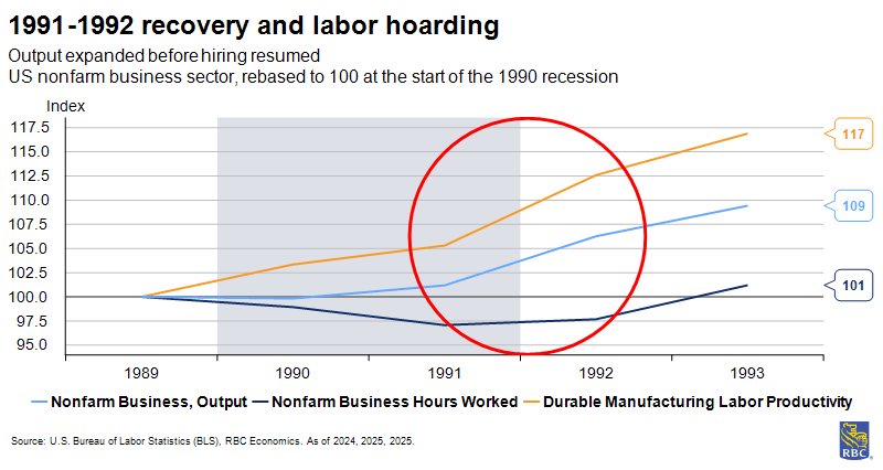
Labor hoarding, the deliberate retention of workers beyond what current output requires, is rational when hiring and training costs are high, and the expected recovery is not too far away. The productivity consequence is that measured output per hour (productivity) falls, because the denominator (hours worked) is declining more slowly than the numerator (real output). Workers are present and on payroll, but not fully utilized.
This tends to be most pronounced in manufacturing, where skilled labor is highly valuable. A plant may retain its core machining and engineering staff through a downturn while cutting the variable and lower-skilled workforce. This pattern produces a measurable productivity decline that reverses sharply once production resumes.
An example of this would be the 1991-1992 recovery—productivity growth accelerated sharply when output expanded while the hoarded workers were gradually put to work (without equivalent new hiring as they were already on payroll).
Similar forces played out towards the end of the pandemic. The national summary section of the Beige Book began to describe firms’ challenges in bringing employees back to work as early as May 2020. By the end of 2021, more than half of firms seeking to hire described the eligible pool as very tight. Once the growth rate moderated, firms were afraid of layoffs as it would have been difficult to rehire staff if the slowdown proved shorter than expected.
Survey data from the National Federation of Independent Business shows that beginning in 2022 firms expected devastating business performance, and simultaneously, expanded headcount and wages. Bound by this mentality, firms varied the number of hours for workers already on their payroll to adjust production rather than decreasing headcount.
When output outlast hours: Worker composition effect
Recessions do not impact all workers equally, and the types of workers who lose jobs matter for the calculation of aggregate productivity.
Job destruction is traditionally concentrated among lower-wage, lower-skill, and lower-productivity workers (often in cyclically sensitive industries like construction, hospitality and leisure, retail), and among workers with part-time status. When these workers exit the measured workforce, the remaining employed population is, on average, more productive.
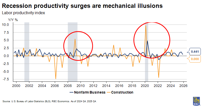
Underperformers are more likely to be culled than those punching above their weight, and a recession acts as the required catalyst. Measured aggregate and industry output per hour can, in these sectors, therefore, rise mechanically during severe recessions. But, not because any worker became more efficient. Instead, the composition of who is working shifted toward higher productivity individuals.
The construction sector’s measured productivity improvement during downturns is the prime example of this mechanism in the sector-level data. However, the strength and direction of the composition effect depends on which workers are displaced and how quickly output adjusts.
During the Global Financial Crisis, for example, other factors obscured or offset the expected composition gains. Worker composition can also operate in the reverse direction during expansions. As the economy recovers and employers reach into the pool of available workers, those with less experience or skills mismatches reentering the workforce reduce the average productivity measure even as the true productivity of workers is no less than it was before.
From aggregate to industry: How the BLS disaggregates
For aggregate measures, BLS uses value-added output: The contribution of production inside the definition being studied (nonfarm business sector, business sector) with all intermediate inputs netted out.
The approach differs when aggregating just at the industry level; removing all intermediates discards information that describes how efficiently the industry transforms what it buys into what it sells. Therefore, in the sectoral (industry) output concept, the BLS includes the value of all goods and services sold to other industries but excludes only the intermediate inputs produced and consumed within the same industry.
The central challenge of industry-level productivity measurement is that different sectors produce fundamentally different types of output, and measuring real output requires, first, defining what the output is and, second, converting its nominal dollar value into a real quantity using the appropriate price deflator. The BLS and BEA solve these problems differently for each sector, and a variety of unique situations related to sectors impact how productivity is measured, evolves, and its outlook.
Manufacturing and construction: Tangible output
Manufacturing is the simplest case; it produces countable units (e.g., automobiles, steel sheets, etc.) with market prices that can be tracked over time to construct output deflators. Quality adjustments are applied to account for improvements, for example in fuel efficiency, embedded electronics, safety features, etc., all of which are imperfect but still anchored to the physical outputs of the sector.
Construction measurement starts from the same physical output premise but encounters a methodological obstacle in its deflation approach. Different projects (hospitals, bridges, data centers) cannot be easily priced on comparable unit bases, so the BLS and BEA rely on more general price indexes to convert nominal construction spending into real output.
These construction price indexes are input-cost based and often do not include quality adjustments for nonresidential structures. Because of this, if input costs and nominal output rise together, the deflator records zero real output growth, even if what was built was more complex and durable than its predecessor, meaning quality improvements often invisible.
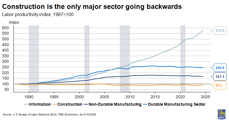
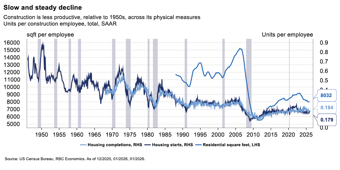
This is one cause of construction’s extraordinary 30-year measured productivity decline. Physical unit measures (e.g., homes per worker, square footage per worker) confirm the same downward trajectory, meaning that the decline exists beyond incomplete quality measurement.
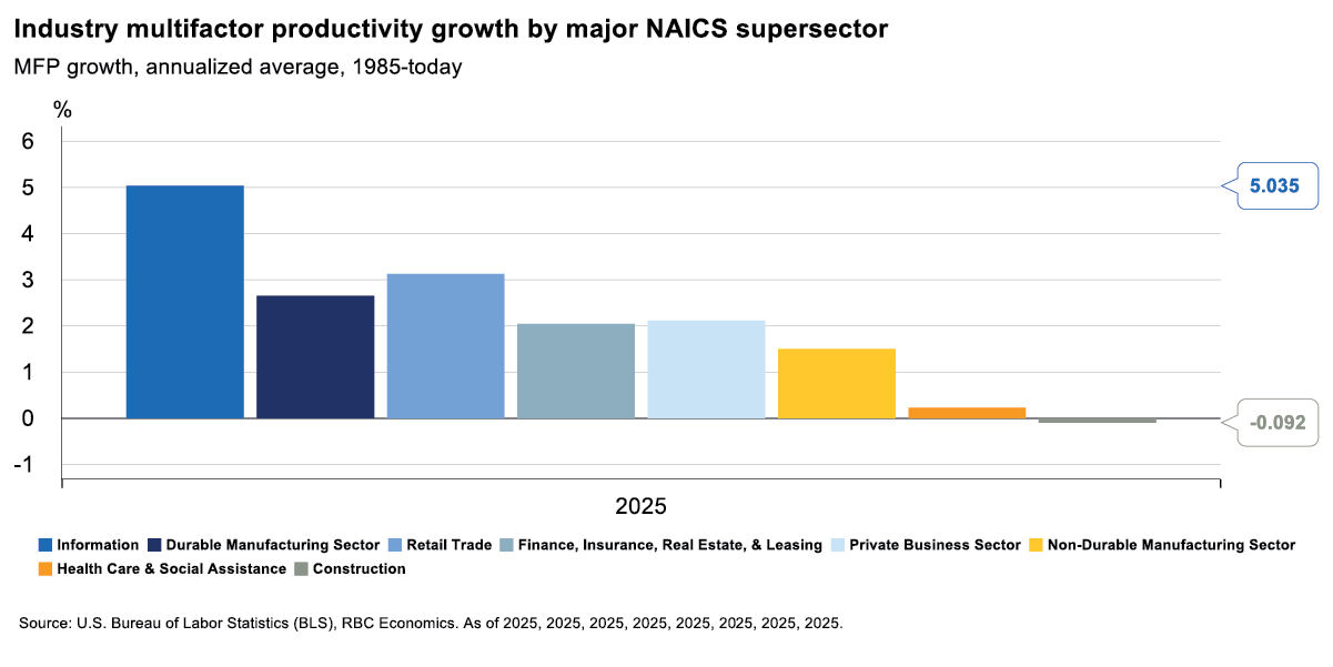
Information: Heavy on the quality adjustments
The Information section contains software publishing, telecommunications, various media industries, data processing, and internet services. On an annualized basis between 1985 and today, its measured productivity growth has been among the highest of any sector. When computing performance doubles at the same price, a naïve deflator (no quality adjustments) would record flat prices and flat real output. Instead, the price of a computing product is comprehensively decomposed into its measurable performance attributes (speed, memory, storage) and the index is adjusted for quality improvement. A data center (or CPU, GPU) capable of twice the compute at the same nominal price records as a 50% price decrease. These adjustments are relatively comprehensive and cover many dimensions of quality.
This is logical as the economy genuinely receives more compute per dollar, but it makes the information sectors productivity figures incomparable with sectors where quality adjustments are less thoroughly applied. A secondary situation applies to this sector: The largest free digital services like search, navigation, social networks, and instant messaging generate enormous consumer value that does not wholly appear in GDP, as the value these services deliver to users vastly exceeds the advertising revenue that represents them in GDP. It is estimated that the consumer surplus from these services is in the hundreds of billions of dollars annually. If these are the most productive outputs of the sector, their exclusion massively understates their contribution to productivity. Therefore, Information is simultaneously understated (free-services exclusion) and overstated (quality deflation applied more aggressively than elsewhere) in terms of productivity.
Retail Trade: Reallocation as Productivity
Retail output is calculated as nominal revenue and deflated with the appropriate merchandise price index. The interesting story is not about the measurement method itself but about what the productivity trend represents. US retail productivity growth in the 1990s, when decomposed, came mainly not from within-firm efficiency improvements but from market share reallocation. Large format department stores, operating at output per hour 40 to 50 percent above the sector median, displaced smaller, less productive independents. The aggregate series rose without much improvement in firm operations mainly because the composition of who was operating shifted towards higher-productivity formats.
The same trend is now operating via the popularity of e-commerce.
E-commerce presents a measurement complication; the BLS CPI for retail merchandise is constructed from in-store price surveys, while online prices for identical products demonstrate higher variation and generally lower prices. In this situation, the deflator used upon e-commerce revenue understates actual price declines and real output growth in the online channel may be moderately understated.
Health Care: Partially Intangible Output
Health care produces tangible outputs as well as intangible, yet very real, outputs like improved health, reduced disability, and longer lifespans. The BLS therefore measures health care outputs using volume proxies – the count of physician services, inpatient days, count of surgical procedures, and prescriptions dispensed. These proxies are unable to capture quality improvements.
About the Authors:
Mike Reid is Head of US Economics at RBC. He is responsible for generating RBC’s US economic outlook, providing commentary on macro indicators, and producing written analysis around the economic backdrop.
Carrie Freestone is a Senior US Economist at RBC. Carrie is responsible for projecting key US indicators including GDP, employment, consumer spending and inflation for the US. She also contributes to commentary surrounding the US economic backdrop which she delivers to clients through publications, presentations, and the media.
Imri Haggin is an US Economist at RBC, where he focuses on thematic research. His prior work has centered on consumer credit dynamics and treasury modeling, with an emphasis on leveraging data to understand behavior.